The neural substrates of general cognitive ability based on multiple cognitive tasks
2023-06-30
Diagram of g and its Relatives
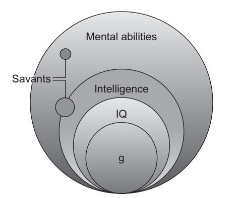
Conceptual relationships among mental abilities, intelligence, IQ, and the g-factor (The intelligent brain, 2013)
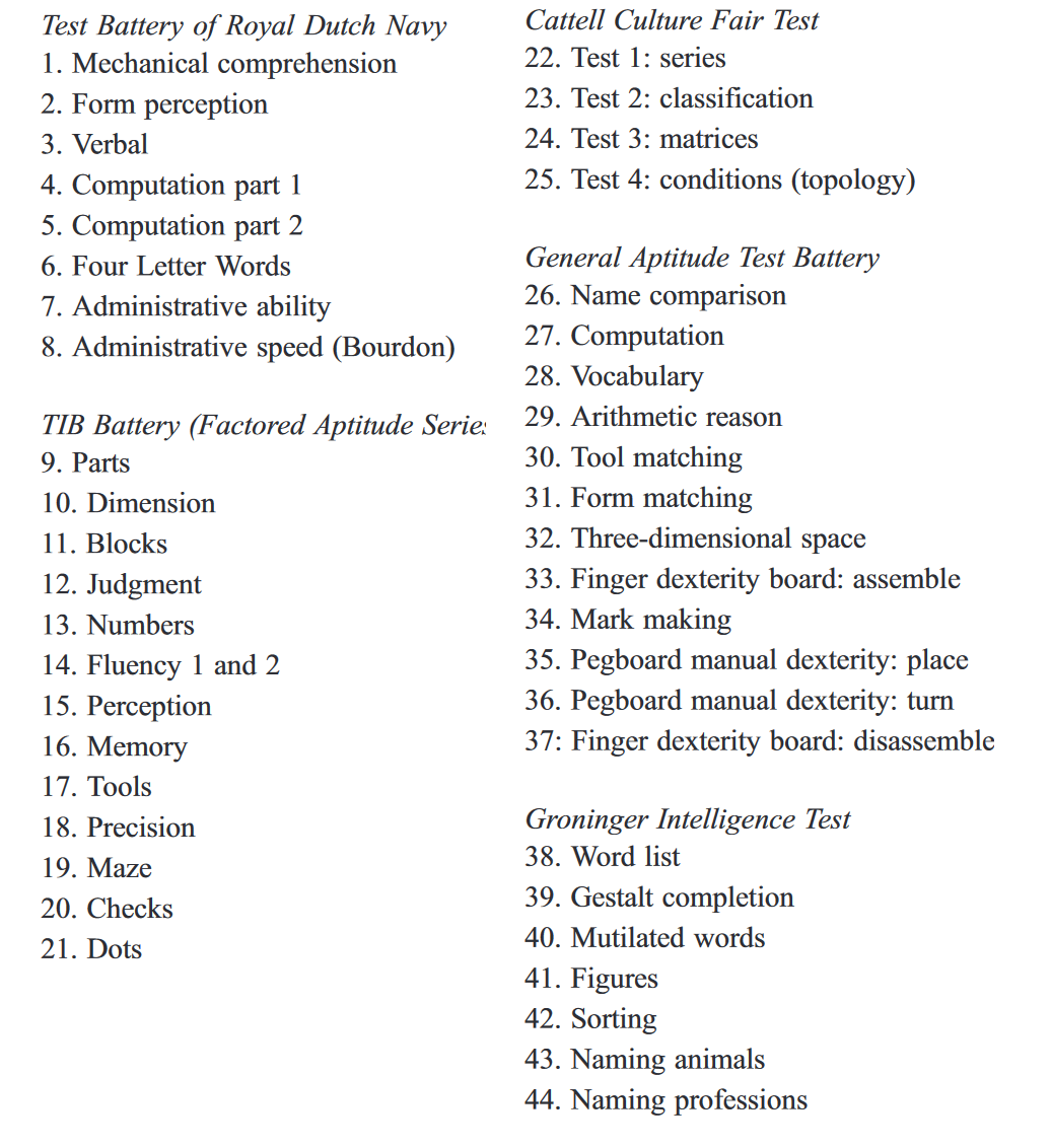
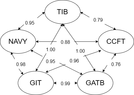
Invariance of g
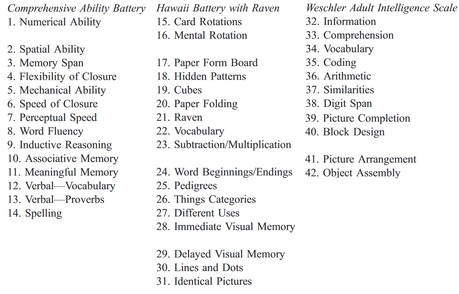
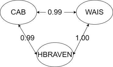
Invariance of g
Explained Variance
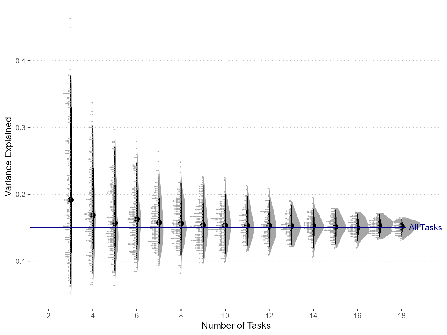
Figure 1: Variance Explained by the g Factor. The horizontal line gives the variance explained by the g factor estimated from all the tasks.
Correlation with RAPM
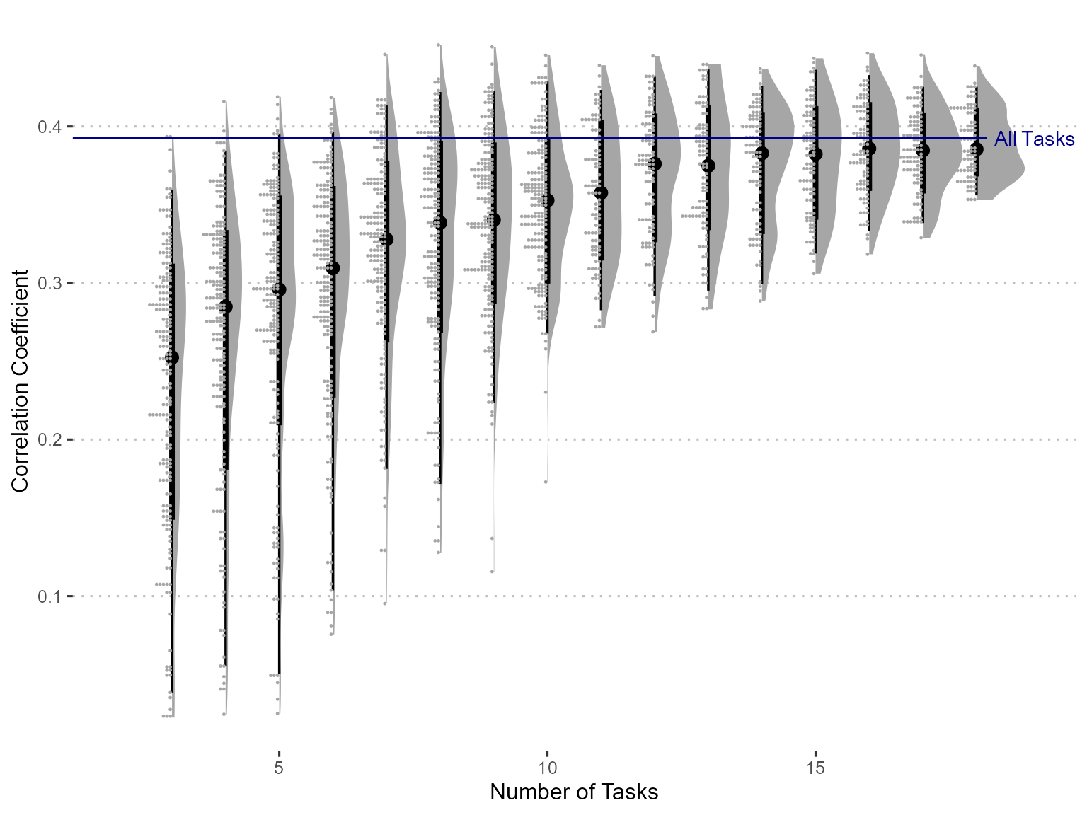
Figure 2: Correlation with Raven’s Advanced Progressive Matrices (RAPM) scores. The horizontal line is the correlation between gF score estimated from all task indices and RAPM.
Correlation between estimated g in Pairwise Sampling
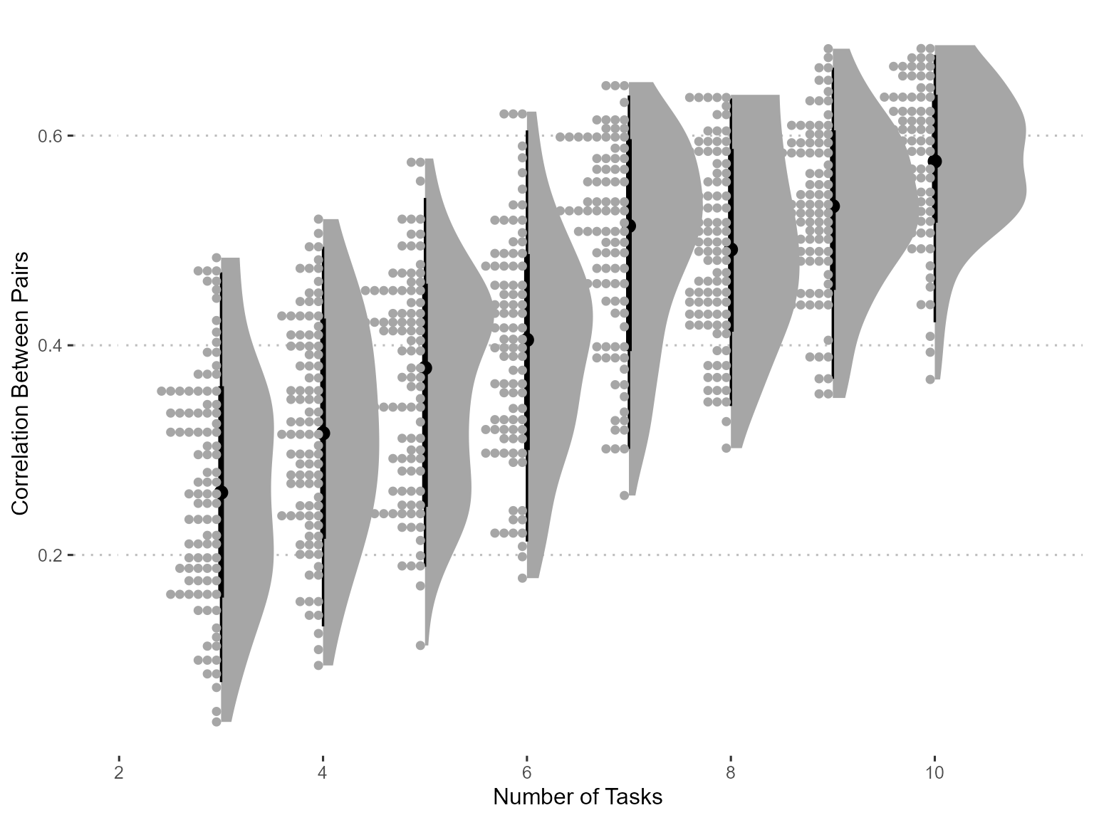
Figure 3: The correlation between g scores estimated from each pair of sampling. For each sampling, a pair of equal-number tasks are drawed without replacement. So the maximal number of tasks will be 10, and this figure shows that the correlations between the paired g scores increase as the number of tasks increase.
CPM hyperparamters checking
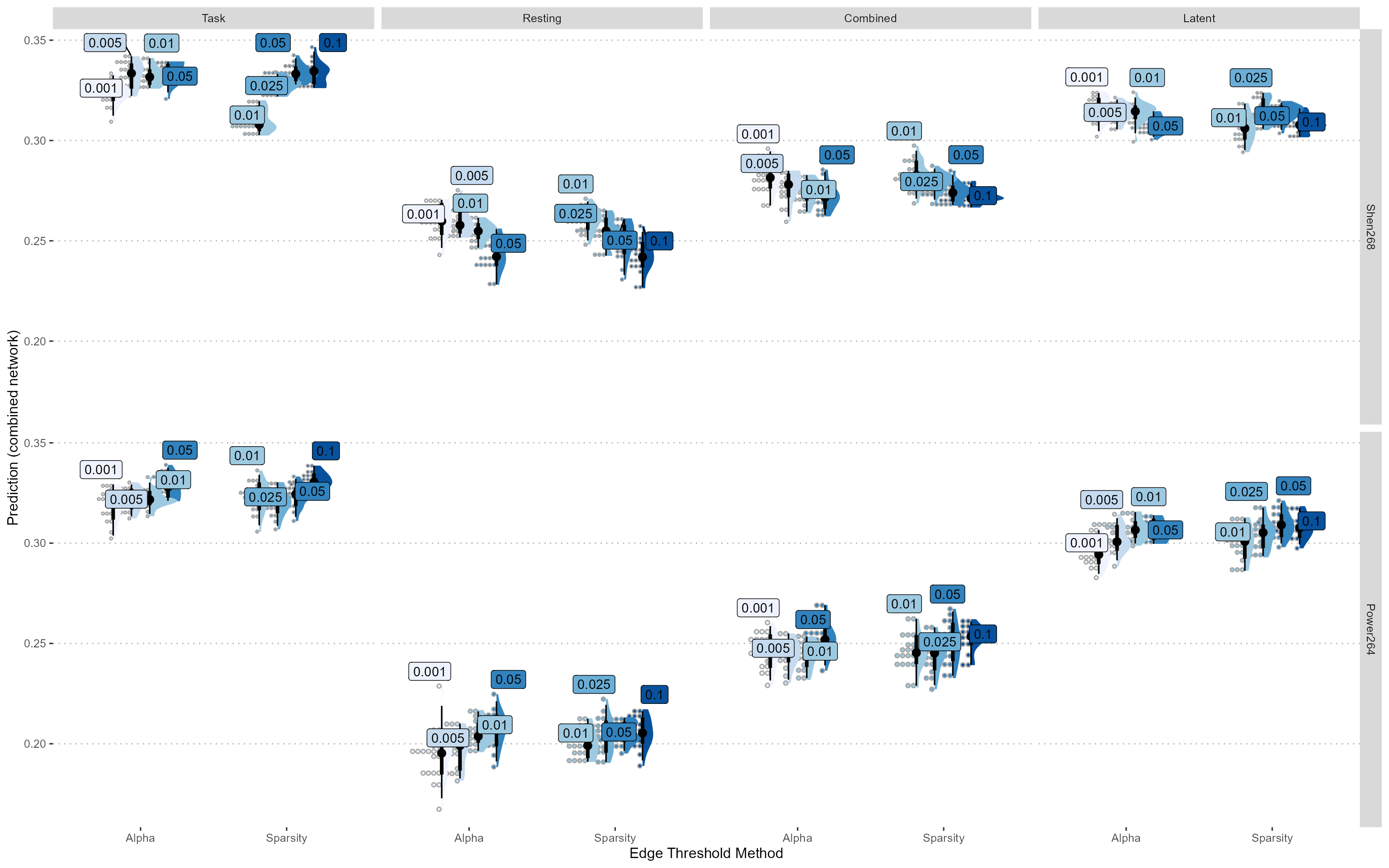
Figure 4: Compare different CPM hyper-parameters. We chose a threshhold method based on alpha level of correlation and a threshhold level at 0.01.
Find the best task condition to predict intelligence
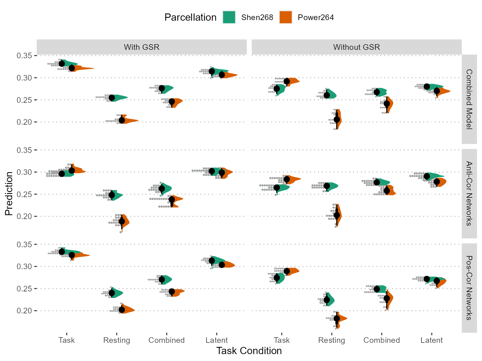
Figure 5: Using CPM method to predict Raven score by FC from different states, we found that task-induced (i.e. n-back task) showed best performance, though combing task and resting states using the first principal component showed comparable performance. What’s more, global signal regression will enhance the performance, whereas different parcellation showed comparable performance.
Prediction Trending
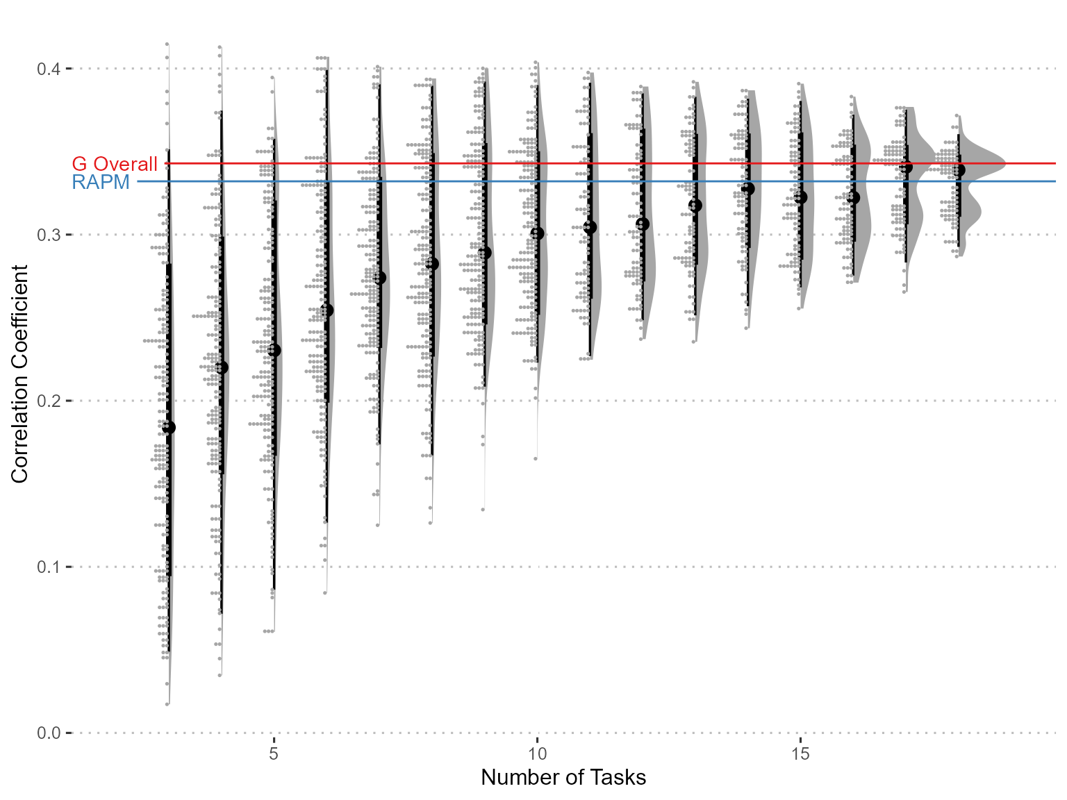
Figure 6: Prediction Trending (based on CPM).
Similarity Between Predictive Network of Pairs
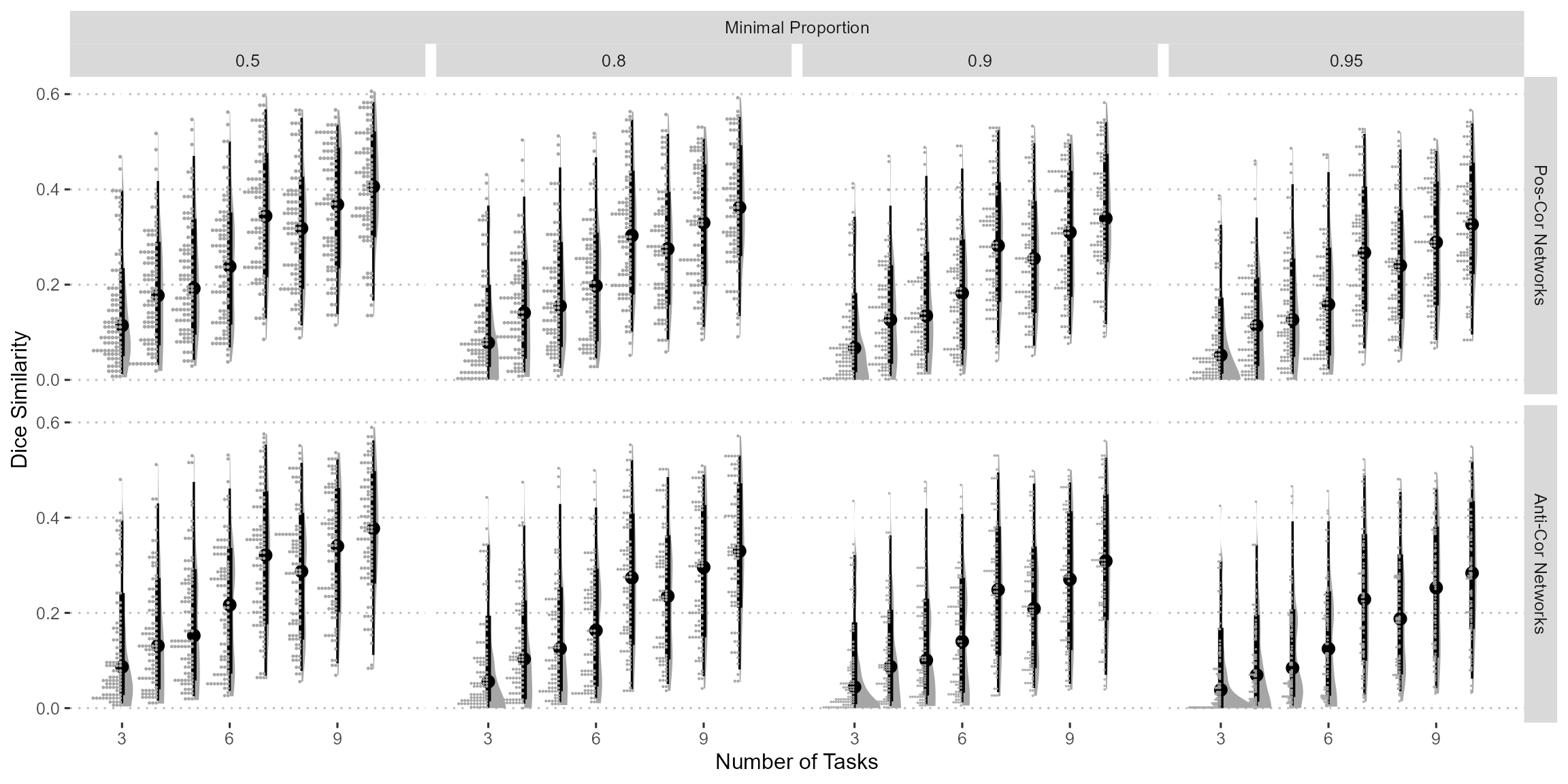
Figure 7: Dice coefficient between each pair of predictive network in pairwise sampling. The edges are kept when given proportion of resamples selected. Here only the results from task state are shown.
Similarity Between Predictive Network of Pairs
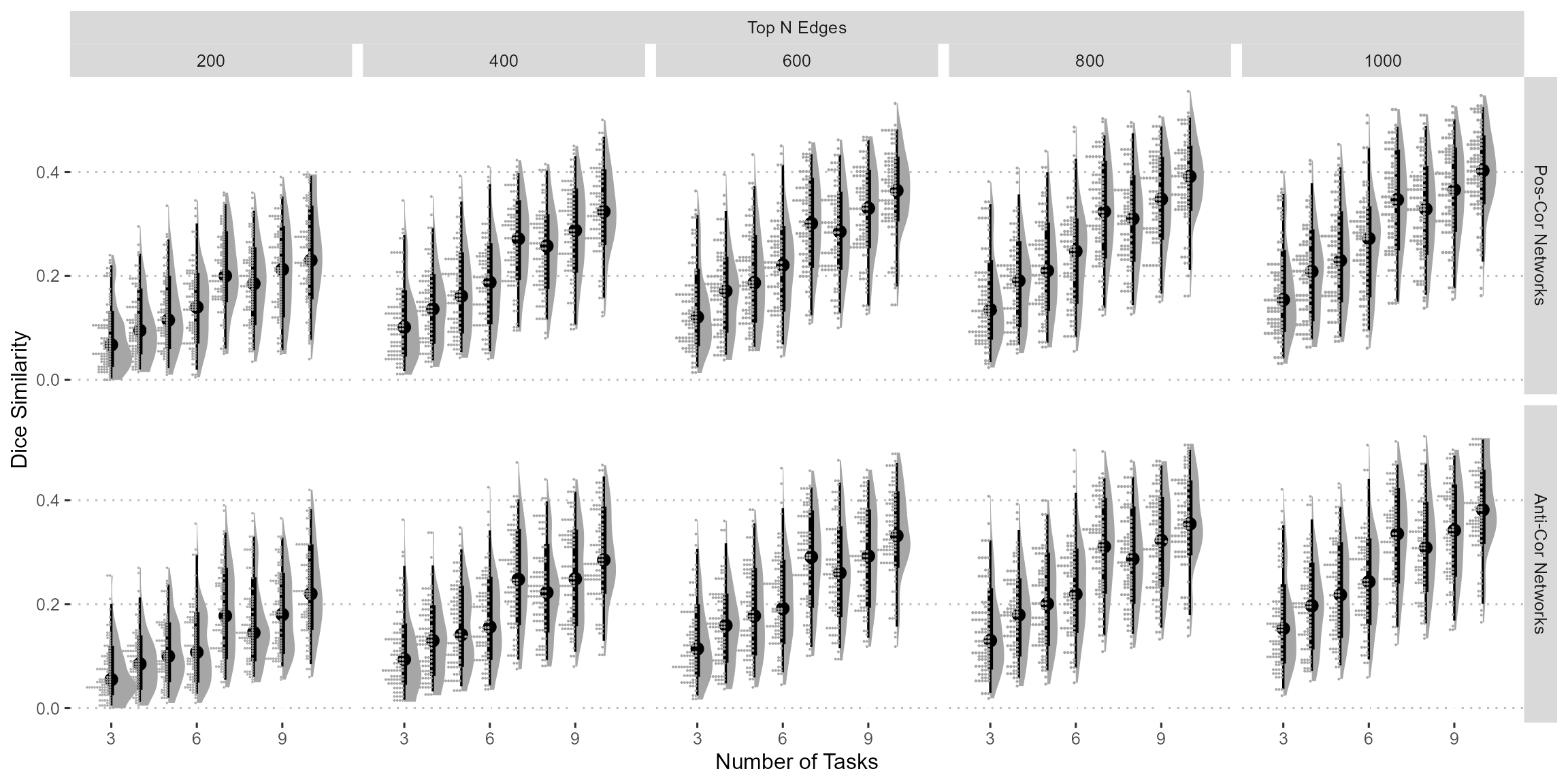
Figure 8: Dice coefficient between each pair of predictive network in pairwise sampling. Only the most selected of given number of edges are kept. Here only the results from task state are shown.
Trends by Number of Kept tasks

Figure 9: The correlation between g factor scores and brain functional connectivity reaches plateau after 6 variables of largest factor loading were included, whereas that of RAPM scores reaches plateau after 13 variables. This might indicate that more variables might not necesssarily be beneficial to the measure of g-factor estimation, esp. when adding low g loading tasks.
Single Task Benchmark
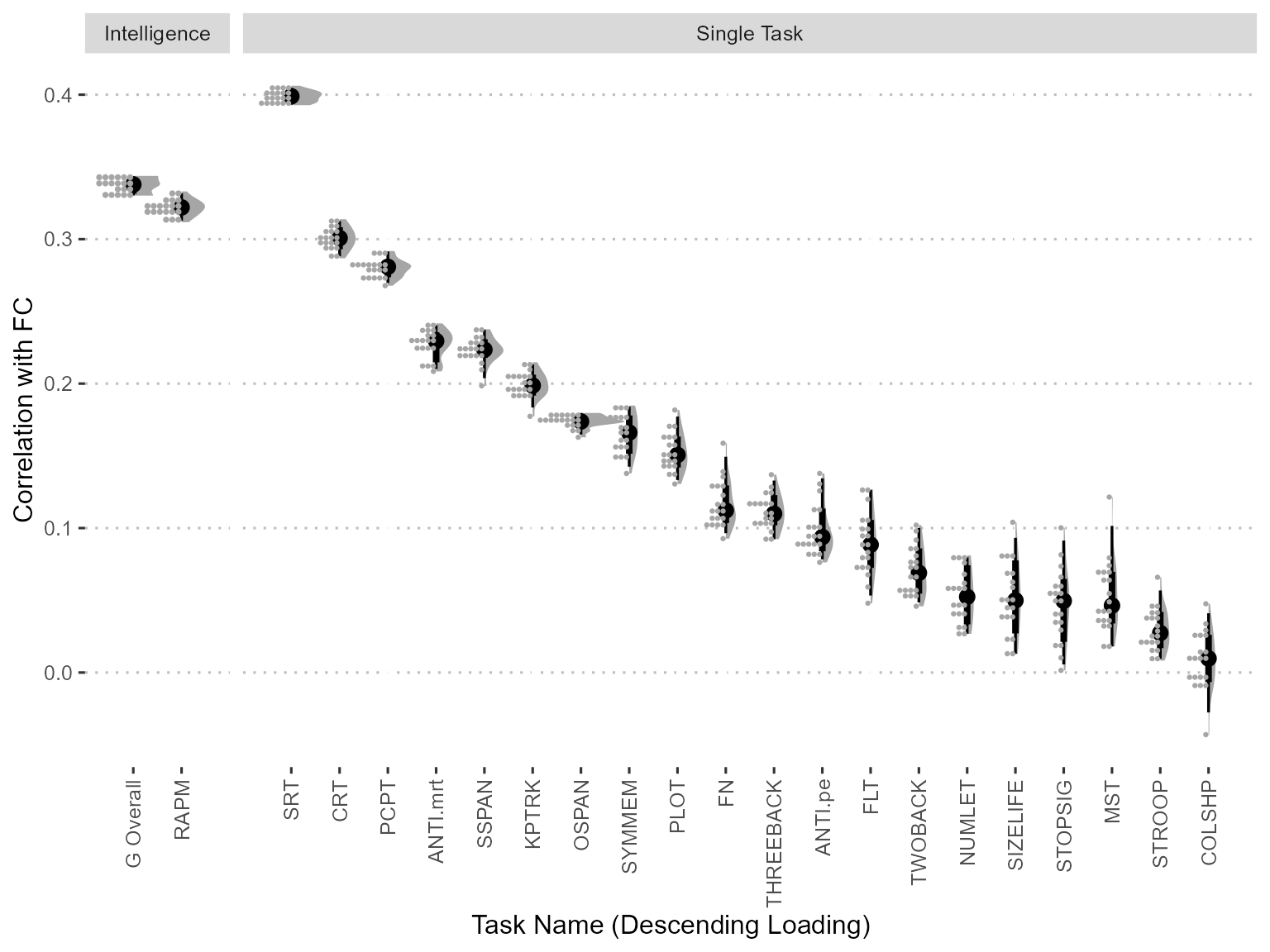
Figure 10: Correlation with brain FC for single tasks. The tasks are ordered by the factor loading in one g factor model.
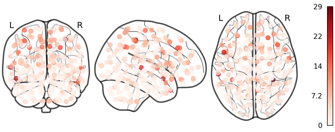
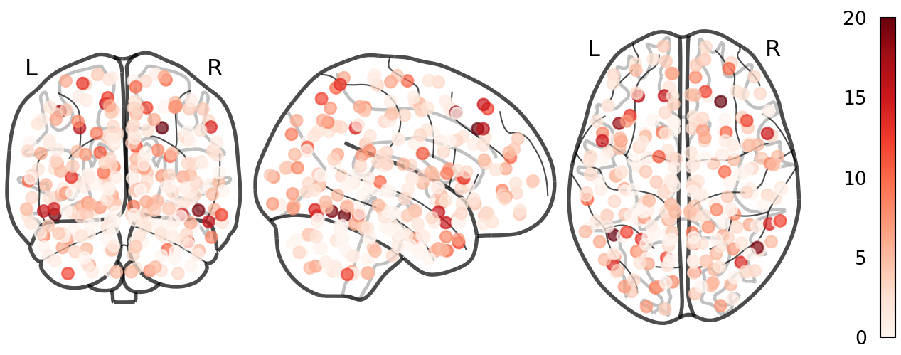
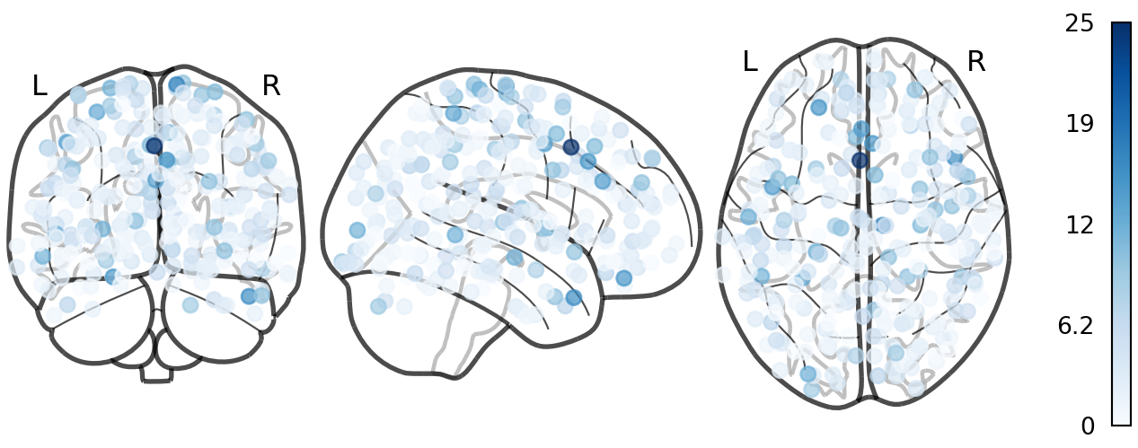
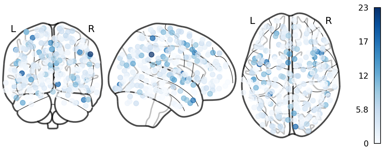
Node Degree (Shen268)
Chord Diagram (Shen268)
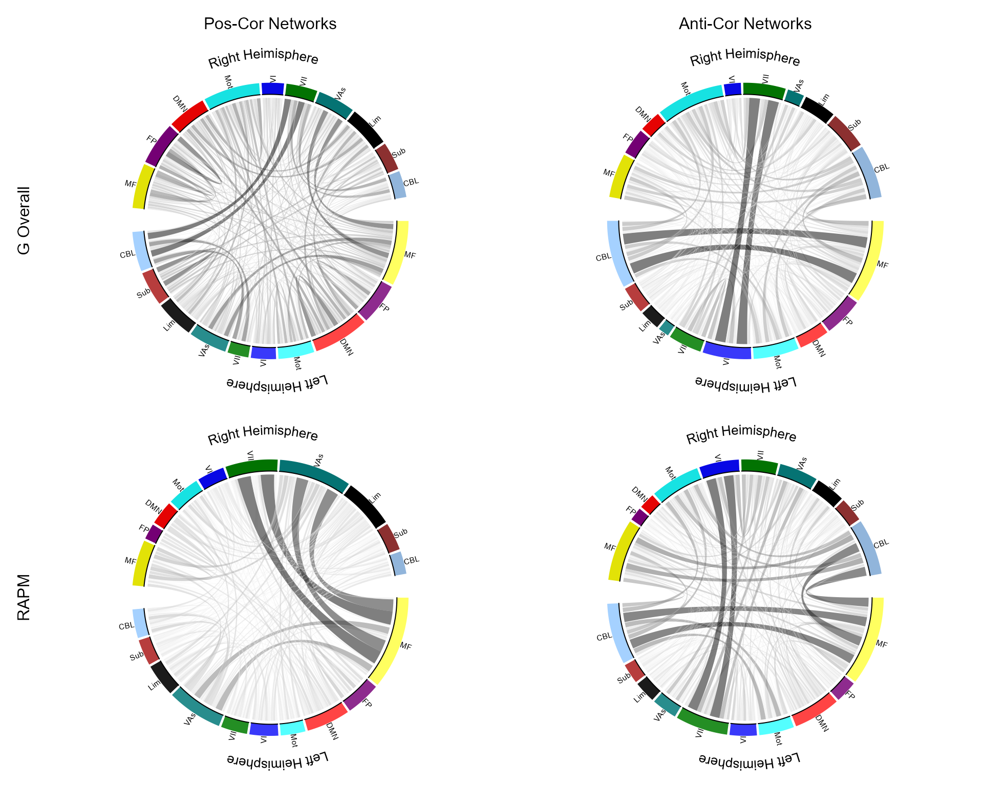
Figure 12: Chord diagram of top 500 edges
Network Contribution (Shen268)

Figure 13: Contribution of Networks
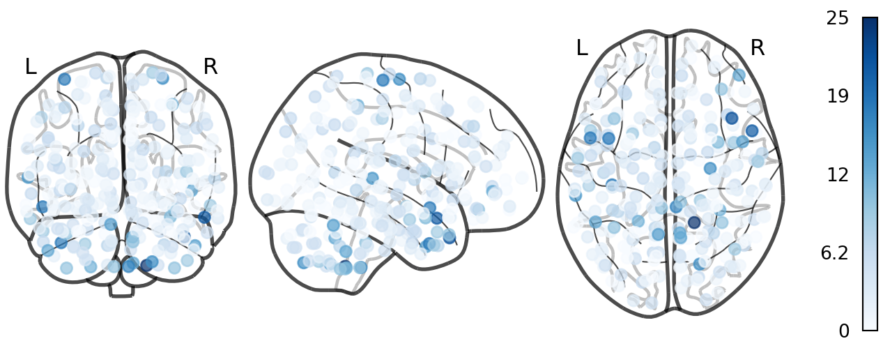
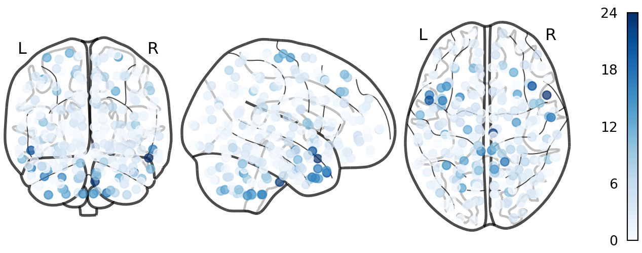
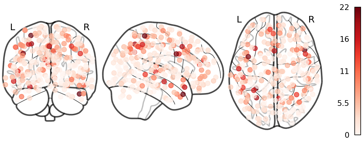
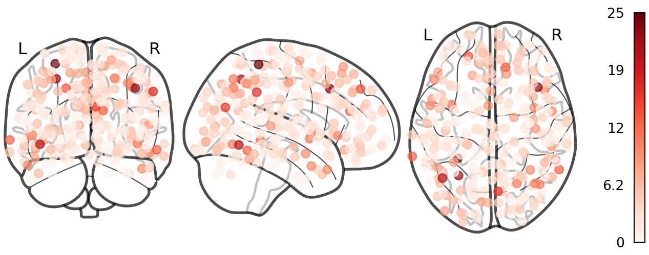
Node Degree (Power264)
Chord Diagram (Power264)
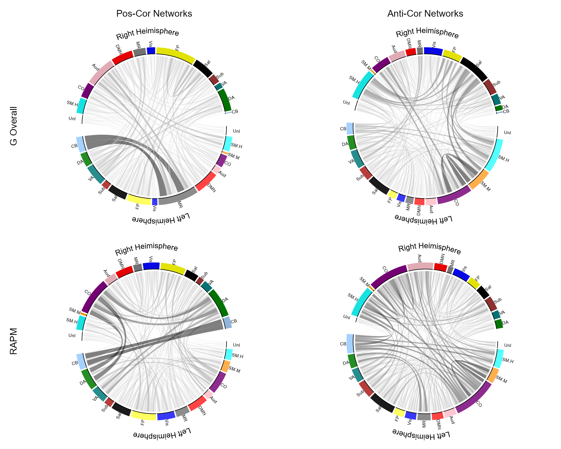
Figure 15: Chord diagram of top 500 edges
Network Contribution (Power264)
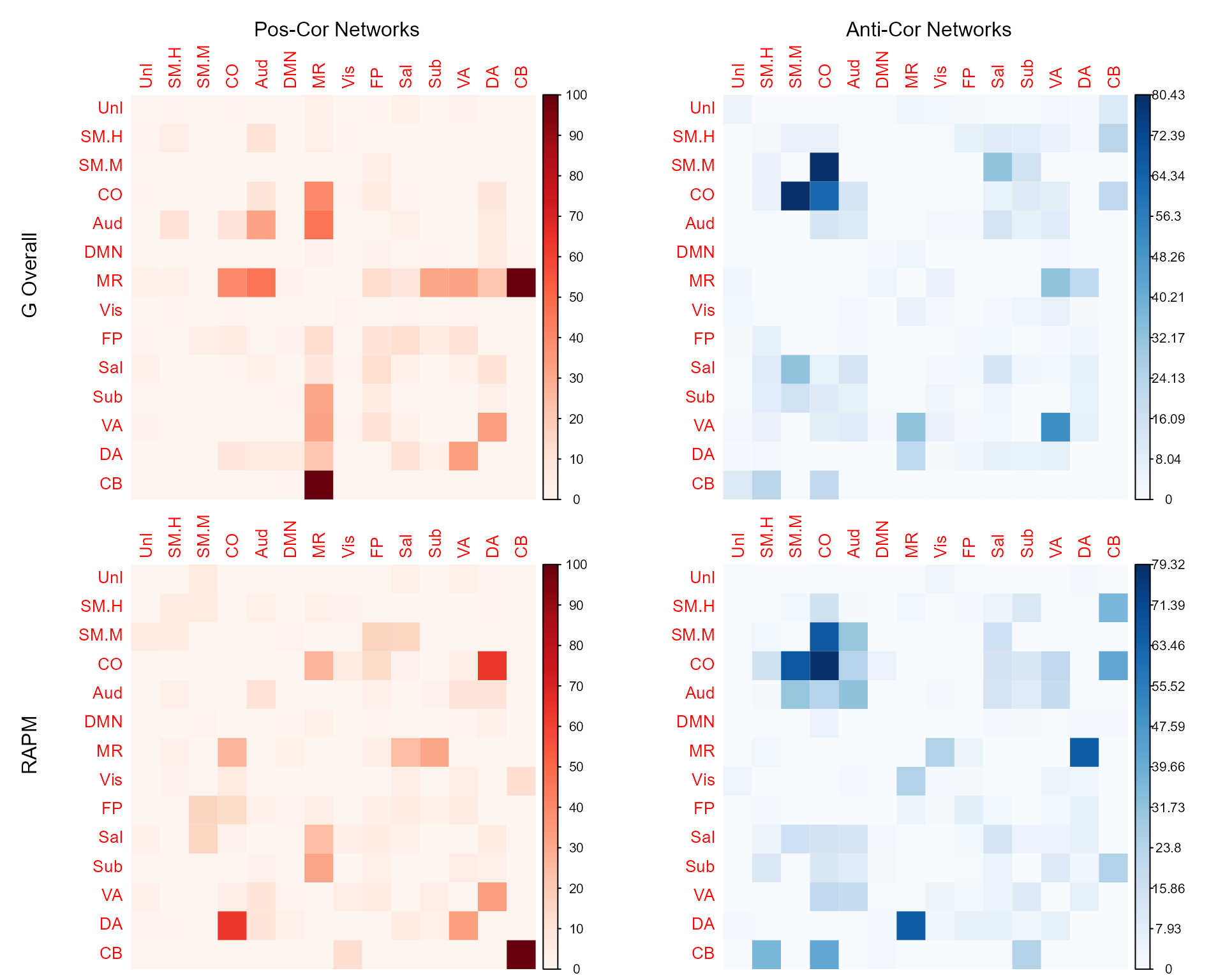
Figure 16: Contribution of Networks